The process of developing a trading strategy (I mean the trading logic, not the application) is an infinite loop:
- Suggest a hypothesis.
- Code it.
- Run a test.
- If the result is not satisfactory, tweak the parameters and repeat.
- If nothing helps, look for an alternative hypothesis.
The question is: what kind of application shall we use for testing in step 3?
Of course, we could use our existing trading app, draft some strategy logic, and then run it in test mode, as we’ve just done, collecting orders and analyzing the equity time series. But then a single test may take days, weeks, and even months if we want to test the strategy under different market conditions. Do you think it’s a bit too long? I agree. That’s why, for research and development purposes, we use backtesting.
We discussed backtesting in Lesson 2, Using Python for Trading Strategies, in the Paper trading, and backtesting – an essential part of systemic trader’s risk management section. In essence, instead of emulating the execution of orders using live data streams, we emulate the data stream itself using pre-saved historical market data. In this case, we can dramatically speed up the testing because computers can process dozens of thousands of ticks or bars per second, compressing months of live testing into minutes or seconds of backtesting. Of course, due to its nature, backtesting cannot guarantee the future performance of a strategy, just because it tests using past data. But regardless, it helps us understand the strategy’s behavior under various market conditions. Generally speaking, if a backtest shows that the emulated equity was mostly growing in the past, then we may suppose that it continues growing in the future, and vice versa: if we saw that the emulated equity was only decreasing over time, or oscillating around zero at best, then we should be very cautious with such a strategy as it’s hard to imagine why it would suddenly start making money when put to production.
I hope you got the idea: we are going to run our code using saved data, not live, so we can process 1,000 or 10,000, or even more seconds of historical data in 1 second.
Now, I believe you will appreciate the approach we followed when developing our code: if you have pre-saved tick historical data, then all you need to do is modify the only function – the one that receives ticks from the data provider – and have it receive data from a local file.
That’s it.
Isn’t it impressive? Yes, you can use the same code for both research and production, thus reducing the probability of making an error to almost zero.
However, you can’t always get hold of historical tick data. Moreover, for strategies that use bars with a higher time frame (such as 1 hour, 4 hours, 1 day, 1 week, and so on), it would be a waste of time waiting until our application forms each bar from ticks. So, we may want to make the following modifications to our code:
- It should now be able to read data from a local file instead of receiving it from a data vendor
- It should be able to process already compressed data (bars) without receiving tick data at all
- It should be able to emulate order execution, which may happen within the duration of a single bar (for example, if the strategy bases its logic on 1-hour bars, then we should be able to emulate order execution between hh:00 and hh:59, where hh stands for the hours’ value).
Looking at the architecture of our existing code, it seems like quite a straightforward task. However, there is one caveat.
Do you remember how we used tick data in the existing code? Yes, we aggregated it into bars, but besides that, ticks were served as a system clock that synchronized the components of the entire application. How do we synchronize them in case we don’t use tick data at all?
Here, we can use another method of controlling the execution of threads – using events.
Syncing threads using events
Let’s quickly jump back to the code that we drafted in the Multithreading – convenient but full of surprises section earlier in this lesson. The problem with that code was that each thread was running when possible, thus producing output at random to a certain degree. And we want all three threads to work one by one – t1, t2, t3, and then again t1, and so on.
The threading module in Python provides several very efficient methods to solve the problem of controlling threads. One of them is using Event() objects.
A threading.Event() object is placed inside the thread’s code and it works like a traffic light. It has two possible states: set or cleared. When the event is set, the thread works as normal. When the event is cleared, the thread stops.
Besides just clearing and setting the events, it is possible to instruct the thread to wait until the event is set. In this case, the thread waits for the event and as soon as it’s set again, it resumes working.
If we want threads to run in a particular order, then we should stick to the following guidelines:
- We need as many events as there are threads
- An event controlling a specific thread should be cleared inside this thread but set outside it
Now, let’s make some modifications to the code.
First, we need three events:
f1, f2, f3 = threading.Event(), threading.Event(), threading.Event()In our example, f1 will control the t1 thread, f2 will control t2, and f3 will control t3.
Next, to the very end of the t1() function, we do the following actions:
- We clear the f1 event (which controls the first thread)
- We set the f2 event (which gives the green light to the t2 thread)
- We set thread t1 to wait for the f1 event to be set again
The modified code will look like follows:
def t1():
    while True:
        print('Receive data')
        time.sleep(1)
        f1.clear()
        f2.set()
        f1.wait()
We modify the t2() and t3() functions in the same way (so that each thread controls its next neighbor) and run all three threads:
def t2():
    while True:
        print('Trading logic')
        time.sleep(1)
        f2.clear()
        f3.set()
        f2.wait()
def t3():
    while True:
        print('Processing orders')
        time.sleep(1)
        f3.clear()
        f1.set()
        f3.wait()
thread1 = threading.Thread(target=t1)
thread2 = threading.Thread(target=t2)
thread3 = threading.Thread(target=t3)
thread1.start()
thread2.start()
thread3.start()
Now, we can enjoy the output in the perfectly correct order:
Trading logic
Processing orders
Receive data
Trading logic
Processing orders
Receive data
Trading logic
Processing orders
Receive data
…and so on.
Note
It is possible that for the first two execution loops, the output may still go in an incorrect order: this may happen until two events are cleared and awaited, and only one event is set.
Now that we’re familiar with threading.Event() objects, it’s time to modify our trading application for backtesting purposes. For clarity and ease of use, I will reproduce its entire code here and point to the exact places where we made any modifications.
Backtesting platform with a historical data feed
As always, we start with several imports:
import csv
import threading
import queue
import time
from datetime import datetime
Then, we reuse the same tradingSystemMetadata class and only add three events to the control threads. We name them F1, F2 and F3 (flags):
class tradingSystemMetadata:
    def __init__(self):
        self.initial_capital = 10000
        self.leverage = 30
        self.market_position = 0
        self.equity = 0
        self.last_price = 0
        self.equity_timeseries = []
        self.F1, self.F2, self.F3 = threading.Event(), threading.Event(), threading.Event()
Next, we need data and order queues. Since we no longer use tick data to sync threads, there’s no need to have multiple tick data queues – we only need one queue for bars and another one for orders:
bar_feed = queue.Queue()
orders_stream = queue.Queue()
Next, we must create an instance of the system metadata object and read the historical data from the file into all_data. We must also start the stopwatch (the time.perf_counter() method) to keep track of time spent on various operations – just out of curiosity.
Note that we read the data using csv.DictReader() so that we receive each bar as a dictionary – this ensures maximum compatibility with the production code that we developed earlier in this lesson:
System = tradingSystemMetadata()
start_time = time.perf_counter()
f = open("<your_file_path>/LMAX EUR_USD 1 Minute.txt")
csvFile = csv.DictReader(f)
all_data = list(csvFile)
end_time = time.perf_counter()
print(f'Data read in {round(end_time - start_time, 0)} second(s).')
Next, we need a modified function that takes bars from the read data one by one, converts necessary fields from str into float, and puts the bar into the queue. We must also break the execution of this loop after the first 10 bars for debugging purposes:
def getBar():
    counter = 0
    for bar in all_data:
        bar['Open'] = float(bar['Open'])
        bar['High'] = float(bar['High'])
        bar['Low'] = float(bar['Low'])
        bar['Close'] = float(bar['Close'])
        bar_feed.put(bar)
        counter += 1
        if counter == 10:
            break
        System.F1.clear()
        System.F2.set()
        System.F1.wait()
    print('Finished reading data')
Note the three flags (System.F1, System.F2, and System.F3) at the end of the function: they control the execution of threads and make sure that first, we read a bar, then we generate an order and, finally, we execute – or, rather, emulate – the execution of this order.
Also, note that we do not check data consistency and do not exclude any data points: when we work with saved historical data, we assume this data is already clean.
Next goes the tradeLogic() function. The best news here is that its main logical part remains completely unchanged – no modification is required between the trade logic starts here and trade logic ends here comments in the original code! We only modify this function at its beginning and at its end.
At its beginning, we must add a try…except statement that will terminate the respective thread when all the data has been processed. To do that, we must set the timeout attribute of the get() method to 1. This means that get() will wait for 1 second for a new bar to appear in the queue, and if no bar is there after 1 second, then an exception is generated. On exception, we just break the loop and effectively terminate the thread:
def tradeLogic():
    while True:
        try:
            bar = bar_feed.get(block=True, timeout=1)
        except:
            break
        ####################################
        #     trade logic starts here      #
        ####################################
        ####################################
        #       trade logic ends here      #
        ####################################
        bar_feed.put(bar)
        System.F2.clear()
        System.F3.set()
        System.F2.wait()
We omitted the entire trade logic because it is indeed identical to what we used in our first version of the trading app.
Note that at end of the function code, we return the bar into the queue: its data will be required by the orders processing component. And as in the case of the previous function, we set the F3 flag, giving the green light to the next operation (orders processing), clear F2, and stop the trade logic thread until the F2 flag is set.
Next, we must rewrite the order execution emulator quite substantially: the difference between the production and backtesting versions is that while backtesting, we only work with compressed data, so checking order execution on every tick no longer makes sense.
Emulating order execution during backtesting
Let’s start by emulating market orders since they’re the easiest to implement, and stick to the following guidelines:
- We assume that a market order can be generated by the trade logic only at the bar’s closing time
- We emulate the execution of a market order only at the bar’s closing price
- We assume that the liquidity in the market is always sufficient and therefore we don’t have to check it before executing an order
- We assume that the actual execution price was the same as the requested order price as we don’t have real-time tick data to test the execution
With all these considerations in mind, the modified emulateBrokerExecution function will now look much simpler:
def emulateBrokerExecution(bar, order):
    if order['Type'] == 'Market':
        order['Status'] = 'Executed'
        if order['Side'] == 'Buy':
            order['Executed Price'] = bar['Close']
        if order['Side'] == 'Sell':
            order['Executed Price'] = bar['Close']
We do not add any flags here as this function is called from inside the processOrders function. Let’s add this function: you will see that its logic looks very much like the one we used previously, with live tick data:
def processOrders():
    while True:
        try:
            bar = bar_feed.get(block = True, timeout = 1)
        except:
            break
We started with a similar try…except statement that terminates the execution of the thread when there’s no more data in the bars queue. Next, we make the same updates to the system metadata as we did previously; the only difference is that we use the bar’s closing price instead of the last tick price:
        System.equity += (bar['Close'] - System.last_price) * System.market_position
        System.equity_timeseries.append(System.equity)
        System.last_price = bar['Close']
The orders processing logic is again quite similar to the tick-driven code, with the main difference being the absence of risk management checks (whether we have sufficient funds to trade) and rejected orders handling: during backtesting, we assume that all orders are executed:
        while True:
            try:
                order = orders_stream.get(block = False)
                emulateBrokerExecution(bar, order)
                if order['Status'] == 'Executed':
                    System.last_price = order['Executed Price']
                    if order['Side'] == 'Buy':
                        System.market_position = System.market_position + order['Size']
                    if order['Side'] == 'Sell':
                        System.market_position = System.market_position - order['Size']
            except:
                order = 'No order'
                break
        System.F3.clear()
        System.F1.set()
        System.F3.wait()
At the end of the function’s code, we again add the respective flags to control the execution order of the threads.
Well, this is it! All we must do now is check the time spent on the backtest (just for fun) and start the threads:
start_time = time.perf_counter()
incoming_price_thread = threading.Thread(target = getBar)
trading_thread = threading.Thread(target = tradeLogic)
ordering_thread = threading.Thread(target = processOrders)
incoming_price_thread.start()
trading_thread.start()
ordering_thread.start()
But how do we check that the code produces correct results?
Of course, we could add several print statements, as we did with the live trading application, but the goal of backtesting is different: we want to process as much data as possible within as brief a period as possible, and then analyze the collected data. 5 years’ worth of 1-minute bars of historical data makes over 2 million data points, so if we just print the updated equity value on each bar, it would make over 2 million prints – which would take forever because print() is one of the slowest instructions. So, how do systematic traders analyze the strategy’s performance?
Equity curve and statistics
When running a backtest with the code we’ve just written, we save some basic statistical data: the equity value updated on every tick or bar. If we plot the equity time series, we get an equity curve: a visual representation of the dynamics of the trading system’s profits and losses over time. Such a chart is the first thing to check after the backtest is complete:
- If the equity curve shows growth over time, then there is a chance (but not a guarantee!) that the strategy may also perform well in the future
- If the equity curve exhibits steady systematical loss over time, it again may not be really bad: consider inverting the rules of the trade logic
- If the equity curve oscillates around zero, it’s probably the worst case as this strategy logic is unlikely to make any money in the future
Let’s add code for plotting the equity curve to our code after the backtest is complete. We will use the techniques that we discussed in Lesson 8, Data Visualization in FX Trading with Python, so I recommend refreshing your memory about using matplotlib at this point.
The matplotlib main loop cannot be run in a thread (at least easily), so we must add charting in the main thread (like we did when plotting live bar charts in Lesson 8, Data Visualization in FX Trading with Python) and keep an eye on the incoming_price_feed thread: while it’s alive, we just wait and do nothing, but as soon as it finishes working, we plot the equity curve.
So, we just add import matplotlib.pyplot as plt to the imports section at the beginning of the code and the following simple infinite loop to its end, once all the threads have been started:
while True:
    if incoming_price_thread.is_alive():
        time.sleep(1)
    else:
        end_time = time.perf_counter()
        print(f'Backtest complete in {round(end_time - start_time, 0)} second(s).')
        plt.plot(System.equity_timeseries)
        plt.show()
        break
If you did everything correctly and used the same historical data file as I did, you will see a chart like the following:
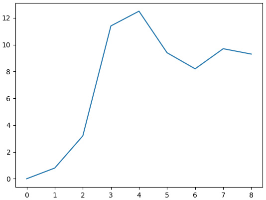
Figure 11.7 – Equity curve of the sample strategy, built on the first 10 bars
This looks great, but how can we make sure that this result is correct? If a backtester emulates the performance incorrectly, we can’t rely on the backtesting results.
Fortunately, it’s not difficult to check this result. As you may remember, we intentionally used a very simplistic test strategy that generates orders on almost every bar. So, we can rebuild a similar equity curve manually, for example using MS Excel or OpenOffice, and compare it with the chart generated by our backtesting app.
Let’s open the data file and remove the unnecessary columns (UpVolume, DownVolume, TotalVolume, UpTicks, DownTicks, and TotalTicks).
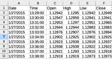
Figure 11.8 – First 10 bars of the source data file
Next, we must reproduce the strategy logic: if the bar closes up (close > open), then we buy; if the bar closes down, we sell. We will add a new column that contains the direction of our trade:
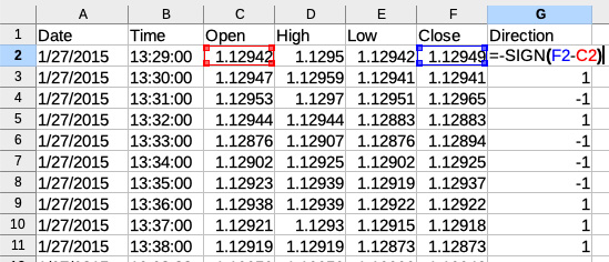
Figure 11.9 – Determining the direction of simulated trade
Then, we must add a column where we calculate the actual PnL per bar by multiplying the difference between the bars’ closing prices by the direction and the trading size:
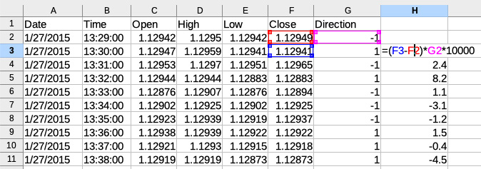
Figure 11.10 – Calculating returns per bar
And finally, we must calculate the cumulative sum of per-bar returns, which is effectively the equity time series:
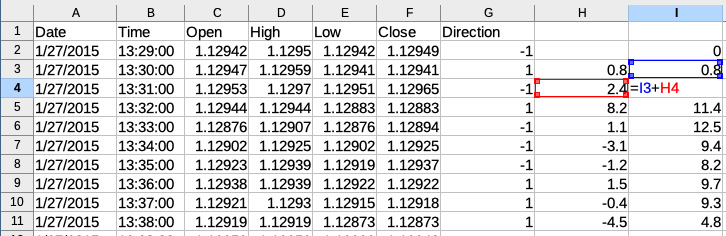
Figure 11.11 – Calculating the equity time series
Now, if we plot the equity curve by creating a line chart based on data in column I, we will see the following:
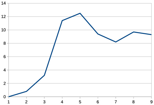
Figure 11.12 – Manual reconstruction of the equity curve in LibreOffice
We can see that the equity curve is identical to what was plotted by our code – and this means that our backtest is reliable! Having checked it only once, we can now trust its results any time we do a test.
I bet you are dying to see a long-term performance report for our great strategy, not limited to just 10 bars. Remember, 1 bar in our source data file is 1 minute, so 10 minutes worth of a backtest is not representative. Let’s run the test for the first 1 million bars, which would equate to approximately 32 months’ worth of history. We only need to modify one line in the code: replace 10 with 1000000 in if counter == 1000000: in the getBar() function.
Now, we also can estimate the backtesting speed as per the output in the console. On my (by far not the latest) laptop (Macbook Pro 2012 with a quad-core Core i7 processor, SSD drive, and 16 GB of memory), it took 12 seconds to read the data from the file and 93 seconds to process 1 million bars. Not bad: we can emulate 32 months in less than 2 minutes!
What about the equity curve from such a long-term perspective? Here you are:
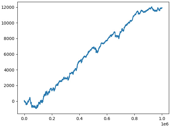
Figure 11.13 – Theoretical performance (equity curve) of the sample strategy calculated using the first 1,000,000 data points
Wow! Looks like the Holy Grail of trading! Is it possible that such a primitive strategy can indeed generate such steady returns over such a long period?
Generally speaking, every time you get such an optimistic result, focus on finding errors. In our case, it is doubtful that we made an error in the trading logic – it’s too primitive and we tested it manually. So, what is it that we probably missed in our backtesting that led to this unrealistically great result? Or maybe this result is indeed realistic?
Of course and unfortunately, it is not.
Let’s go back to the emulateBrokerExecution function again. We assume that any order is executed on the bar’s close – which is fine as we don’t have tick data for backtesting. But our code makes no difference between the execution of buy and sell orders: they are both executed at the same price, in our example – bid. But when testing the live trading application earlier in this lesson, we saw that executing orders at actual prices (bid for sell orders and ask for buy orders) may make quite a difference in PnL. So, as we don’t have ask prices in our historical data, let’s emulate it: we will add a typical spread to the bar’s closing price, thus accounting for the difference between the bid and ask:
        if order['Side'] == 'Buy':
            order['Executed Price'] = bar['Close'] + 0.00005
In reality, the spread in EURUSD may vary from as low as 0 to as much as 0.0010 and even greater (usually before the release of important economic news; see Lesson 6, Basics of Fundamental Analysis and Its Possible Use in FX Trading), but it’s safe to assume that 1/2 pip is more or less adequate to emulate the average spread.
Let’s run the backtest again and see the equity curve:
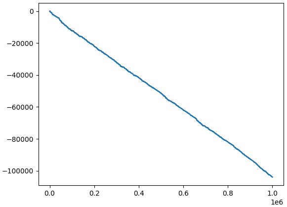
Figure 11.14 – More realistic emulated equity curve of the test strategy
What a radical difference! Now, instead of steadily gaining money, the strategy is steadily losing money, and is doing so very, very quickly: it lost $100,000 in less than 3 years by trading only one so-called mini-lot (10,000 base currency).
How has this happened?
Although the strategy made money on paper without accounting for the spread, on average, it produced a ridiculously small amount of paper money per trade: it was less than the spread. As soon as we correctly emulated the execution of orders at the bid and ask, the Holy Grail vanished into thin air and the sad truth was revealed.
Note
This story should always be kept in mind when you do any market research and develop any strategy. Always make sure that you emulate the real market conditions to the best possible extent – to avoid getting too optimistic theoretical results and quite painful disappointment in production.
The greatest news after all this is that you now have a tool you can rely on: our backtesting platform.
Leave a Reply