This component should be able to receive ticks from virtually any source, clean it up, translate them into the single format used throughout our app, and put them into the data queue:
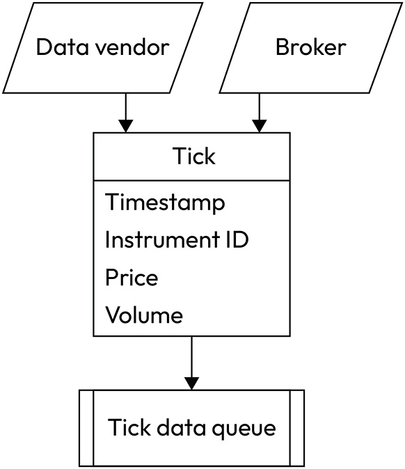
Figure 11.1 – Tick data receiving component
The beauty of this approach is that as soon as the tick is sent to the tick queue, we can forget about it. This process is now isolated from the rest of the app, and should we need to change the data vendor or the broker, we can do that by rewriting the respective module without making a single change in the rest of the code.
Many strategies require tick data. For example, arbitrage strategies (see Lesson 9, Trading Strategies and Their Core Elements) can work using only tick data. However, the majority of trading strategies use logic based on compressed data, not ticks. So, we need to add a component that can aggregate ticks into bars (see Lesson 5, Retrieving and Handling Market Data with Python, the Data compression – keep the amounts to the reasonable minimum section).
Data aggregation component
This module should be able to not only aggregate live tick data into bars. When we develop a strategy, we normally use historical market data stored locally already in a compressed form, so there’s no need to waste time aggregating ticks during a test run. Thus, we must add the following part to our app architecture:
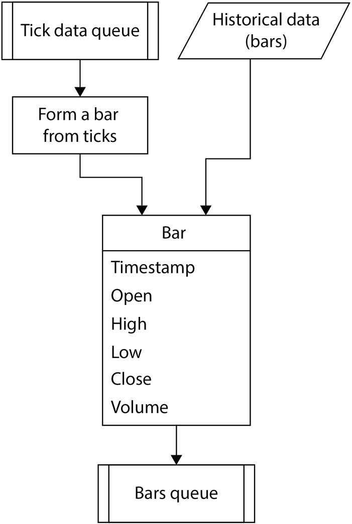
Figure 11.2 – Reading bars from storage or forming bars from ticks
Again, as in the previous case, this process is isolated from the rest of the application, so we can implement it once and forget about it until we need to modify something in the way we aggregate ticks into bars.
Next, we should implement the trading logic.
Trading logic component
This component may use both tick and bar data as input and produce orders as output. This output should go into the order execution control component of our trading app, so it’s quite natural to use another queue again: the ordering queue that would isolate the order execution component from the rest of the application.
However, besides just sending orders out, we need another connection between the trading logic and the order execution components. This connection should provide feedback from the execution of the order to the trading logic. How do we establish such a connection?
The first idea that probably comes to mind at this point is to use yet another queue. However, in this case, it’s not convenient. Queues are great when you want to trigger a certain process as soon as data is in the queue – in other words, they are ideal for event-driven processes. But market position or equity values do not trigger any process by themselves: they are only used by various components of the trading app as auxiliary values. Therefore, instead of a queue, we will create an object that will store all the required data about the implemented trading strategy and share this object across all components of our trading app.
This object can contain any strategy metadata, such as market position, equity time series (see below), running PnL, realized profit or loss, various statistical metrics, and so on:
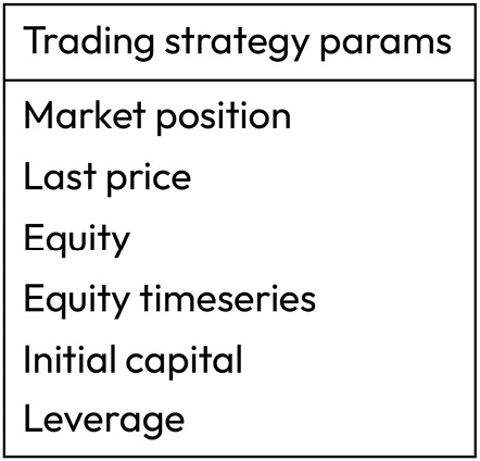
Figure 11.3 – Prototype of an object that stores trading strategy metadata
Last price means the quote received with the previous tick (or bar) and it serves to calculate the running PnL between two ticks (or bars): if the position is long and the price has increased, then the running PnL has also increased, if the position is short and the price has decreased, then the running PnL nevertheless increased, and so on. If we sum all changes in the running PnL on every tick or bar from the moment when the strategy started until the present, then we will get the overall profit and loss, which is frequently referred to by traders as equity. This is a bit of professional slang because formally, the equity is the value attributable to the owners of a business (see, for example, for details), but in algo trading, equity frequently means just the realized profit and loss, plus the value of the open position.
We can also save the equity value on each tick or bar, thus creating a time series. This time series is normally referred to as the equity curve and works as the most common illustration of the trading strategy’s performance: the way the strategy behaved in the past and when and how much money it made (or lost). This information can also be used by the trading logic, along with market price data and market position.
We also included two money management-related parameters: initial capital and leverage. These values can be used to check if we have sufficient funds to trade and also to determine the actual trading size for our orders.
Now that we’ve added such a universal object that transfers strategy metadata between the trading logic and the order execution component, we can add the trading logic component to our architectural diagram:
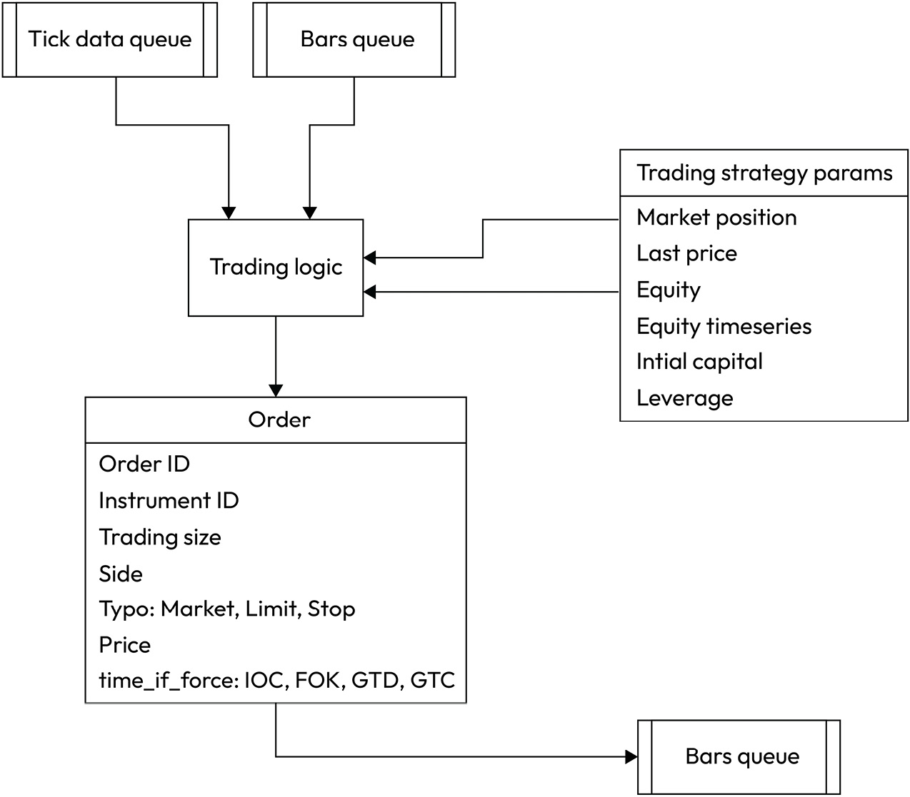
Figure 11.4 – Trading logic and common trading strategy parameters container
The last mandatory component to be added is the order execution component.
Order execution component
This component not only implements an ordering interface with the broker or emulates the execution of orders locally. It will also do some basic analysis of the strategy’s performance – for the needs of the trading logic. It should process the order, send it to a broker or emulate it locally, receive the execution status, process this status (for example, if the order was rejected, decide what to do: cancel or submit again), calculate the running PnL, and build the equity curve. Let’s add it to our diagram:
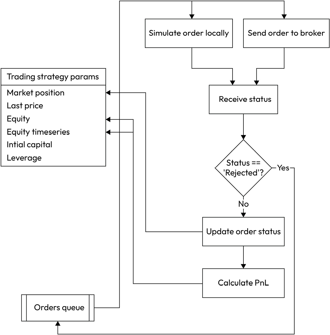
Figure 11.5 – Order execution control module and its interaction with the trading strategy properties object
Let’s see how it works. First, we receive an order or orders from the order queue. These orders were generated and put into the queue by the trading logic. Then, we send an order to the broker or emulate its execution locally and receive the order status. If the order was executed, then we update the PnL and add another data point to the equity time series. If the order was rejected, we return it to the order queue and the whole process starts over automatically.
Note that the strategy metadata (market position, equity, and so on) is updated with every processed order. This ensures the ultimate precision in making trading decisions and controlling the actual market exposure.
Great! We now have a general view of the entire trading app architecture. And the most pleasant thing is that it is split into small, relatively simple components. We know how these components should communicate with each other, we know the data formats, and we know the sequence in which they should operate, so it seems we know everything we need to implement a trading application.
But before we start coding, I’d like to emphasize two advantages of the suggested architecture that are very hard to overvalue.
Advantages of the modular architecture
First of all, this architecture makes sure that your trading app will never peek ahead during the research phase (while using historical data). At this point, I recommend that you refresh your memory regarding peeking ahead, which was considered in detail in Lesson 4, Trading Application – What’s Inside?, in the Trading logic – this is where a small mistake may cost a fortune section – I am sure you will appreciate the suggested architecture of our trading app.
Second, this architecture provides for a flexible modular code that conforms to the concept of a universal trading application: you can quickly switch data sources and trading venues and use the same application both for research and production.
It seems like we have covered everything we need to start coding our first trading application. However, there is one point of extreme importance that is surprisingly too frequently missed by so many developers: the problem of thread synchronization. To understand this problem and find out the right solutions to it, let’s do a brief lyrical digression about multithreading.
Leave a Reply