In Lesson 1, Developing Trading Strategies – Why They Are Different, we proposed a generalized architecture of a trading application. In brief, it consists of the following components:
- Data receiver: Something that retrieves live data from the market or historical data stored locally; see Lesson 5, Retrieving and Handling Market Data with Python
- Data cleanup: A component that eliminates non-market prices; see Lesson 1, Developing Trading Strategies – Why They Are Different
- Trading logic: The brains of the trading app that make trading decisions (see Lesson 6, Basics of Fundamental Analysis and Its Possible Use in FX Trading, Lesson 7, Technical Analysis and Its Implementation in Python, and Lesson 9, Trading Strategies and Their Core Elements), frequently with integrated pre-trade risk management
- Ordering interface: A component that receives trading signals from the trading logic, converts them into orders, and keeps track of their execution; see Lesson 10, Types of Orders and Their Simulation in Python
- Post-trade risk management and open positions management, such as keeping track of the running loss and liquidating losing positions or all positions
Anyway, this simplified architecture lists the essential components but does not say anything about how they communicate with each other. Of course, it is possible to use a linear architecture where all the components are implemented as dependent pieces of code executed one after another in sequence. Such a solution is simple, but has significant drawbacks:
- You won’t be able to add more trading logic components to run multiple strategies in parallel
- You won’t be able to send orders to multiple trading venues
- You won’t be able to receive information about the actual consolidated market position in the trading logic
- You won’t be able to reuse the same code (at least in parts) for both development and production
Let’s stop for a while at these four disadvantages.
Regarding the first two points, you may probably say that you’re not going to run multiple strategies and trade at multiple trading venues as we’re only making our first steps into algo trading, and doing that cross-venue and cross-trading logic is more of an institutional activity. I could argue that, in reality, it’s more than normal for private traders to do all that, but these two points are less important than the remaining two.
To understand the importance of the third point, we have to introduce a new term: consolidated market position.
Imagine that you have several strategies and all of them trade in the same market – say, EURUSD. The first one bought 100,000 euros, the second one sold 80,000, and the third one bought 50,000. Why has this happened? It’s quite a common situation: for example, you run a short-term mean reversion strategy, longer-term breakout, and long-term trend following strategies (see Lesson 9, Trading Strategies and Their Core Elements); they generate trading signals independently, but so long as they all trade the same market, they all contribute to the amount of the asset currently traded. This amount is called the consolidated market position.
In our example, the individual positions per strategy are 100,000 long, 80,000 short, and another 50,000 long, so the consolidated position is 70,000 long. This is your real market exposure and all position sizing calculations should rely on this figure.
But what about the entry price for such a consolidated position?
In Lesson 10, Types of Orders and Their Simulation in Python, we explored the average execution price for an order that was executed in parts. The same approach can be used to calculate the average entry price for the consolidated market position. Let’s do this simple math for our example with three open positions.
Suppose that the first (100,000 long) position was opened at 1.0552, the second (80,000 short) at 1.0598, and the third (50,000 long) at 1.0471. First, we calculate the sum of these prices multiplied by the respective trading size. Don’t forget that short positions (which effectively reduce the consolidated market position) should be accounted for as negative numbers:
S = 100000 * 1.0552 – 80000 * 1.0598 + 50000 * 1.0471 = 73091
Now, we divide the sum, S, by the actual consolidated market position, MP, which equals 70,000, and we get the average entry price:
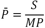
In our example, the consolidated average price is approximately 1.0442. At first glance, it looks ridiculous as it is way lower than the lowest of the actual traded prices. But it’s really easy to make sure it’s correct.
Imagine that the current market price is 1.0523. Let’s calculate the running profit or loss (typically referred to as running PnL or running P/L; see Lesson 3, FX Market Overview from a Developer’s Standpoint, the Trade mechanics – again some terminology section) for each position: it’s just the distance between the current price and the entry price multiplied by the trading size. The first position running PnL at 1.0523 equals (1.0523 – 1.0552) * 100,000 = -$290, the second position running PnL equals (1.0523 – 1.0598) * -80,000 = $600, and the third position running PnL equals (1.0523 – 1.0471) * 50,000 = $260. Thus, for the consolidated market position, the running PnL equals $570.
Now, let’s do the same math with the price and the size of only one consolidated market position. Given it was opened at 1.0442 and the current market price is 1.0523, its running PnL is (1.0523 – 1.0442) * 70,000 = $567, which is not exactly equal to $570 only because we rounded the average price to the 4th digit. So, we can indeed use the average price and the resulting trading size of the consolidated market position instead of calculating the PnL for each position separately.
Note for nerds
Such a consolidated position calculated as the average of all orders with their respective trade volume is often called the Volume Weighted Average Price (VWAP). However, the VWAP is normally only used to evaluate a position that was accumulated by multiple entries to the same direction, and so long as we are discussing the net position as the result of trades taken to both sides, I prefer using consolidated, although it’s not a regular term.
A consolidated market position is extremely important to correctly implement risk management. If you don’t know this position, you have no idea about your running profit or loss, so you don’t know when to liquidate a losing position – which may end up with a disastrous loss. Moreover, you may not know even how much to liquidate, and open a new position instead of only covering a loss.
Even if you run only one strategy in one market, it is no less important to know the exact market position as it exists in the real market: don’t forget that a certain order may not be executed or executed at a price different as expected due to several reasons (see Lesson 10, Types of Orders and Their Simulation in Python). So, if you don’t let your code provide feedback from the broker to the trading logic, you may have a hard time managing your positions.
The fourth disadvantage is hopefully more evident: if we can suggest an architecture that is flexible, modular, and reusable, then it has an advantage over something that should be modified entirely every time you want just to switch a data source.
So, with all these considerations in mind, what can we suggest to make the architecture of our trading app meet all the requirements mentioned?
We already know the solution, and we used it quite successfully in Lesson 5, Retrieving and Handling Market Data with Python. This solution is to use threads and queues to make the components of the app work independently. I strongly recommend that you refresh your memory regarding threads and queues by referring to the Working with saved and live data – keep your app universal section of that lesson.
Now, let’s redraw the app architecture diagram, this time at a bit lower level, closer to the transport layer, not just business logic.
As always, we will start from the beginning: receiving live (tick) market data.
Leave a Reply