As always, we start by doing some imports:
import json
import threading
import queue
from datetime import datetime
from websocket import create_connection
Next, we create a class that contains the strategy metadata (see the Trading logic component section):
class tradingSystemMetadata:
    def __init__(self):
        self.initial_capital = 10000
        self.leverage = 30
        self.market_position = 0
        self.equity = 0
        self.last_price = 0
        self.equity_timeseries = []
Now, we prepare three (!) tick data queues:
tick_feed_0 = queue.Queue()
tick_feed_1 = queue.Queue()
tick_feed_2 = queue.Queue()
Why three? This is one of the solutions to the thread synching problem explained in the Multithreading – convenient but full of surprises section.
The first queue (tick_feed_0) connects the market data receiver with the ticks aggregation component, which forms bars. This component is activated every time a new tick is in the first queue. After the component has finished, it puts the same tick into the second queue (tick_feed_1).
tick_feed_1 connects the ticks aggregator with the trading logic, and the trading logic is invoked only when there’s a new tick in tick_feed_1. But it may enter this queue only after the first component has finished working! So, trading logic cannot be invoked earlier than a new tick is processed. Then, similarly, the trading logic components put the same tick into the third queue (tick_feed_2).
tick_feed_2 connects the trading logic with the order execution component, and this component is invoked no earlier than there’s a new tick in tick_feed_2. So, using three queues to connect components one to another ensures the correct sequence of operations.
Important note
This method of synching threads would work only if the interval between ticks is greater than the round trip time for all threads triggered by it to finish working. This is valid for most data feeds as normally, we receive no more than 10 ticks per second, and the round trip processing time is typically around 0.0001 seconds. This approach won’t work with heavy load exchange market data received via the ITCH protocol, which sometimes receives over 10,000 ticks per second. However, this is specific to institutional trading and we don’t consider solutions of this kind in this app.
Next, we must add a queue to process aggregated market data (bar_feed), a queue to store orders (orders_stream), create an instance of the system metadata class, and specify the parameters required to connect to a data feed (in our example, we use LMAX as the source of market data):
bar_feed = queue.Queue()
orders_stream = queue.Queue()
System = tradingSystemMetadata()
url = "wss://public-data-api.london-demo.lmax.com/v1/web-socket"
subscription_msg = '{"type": "SUBSCRIBE","channels": [{"name": "ORDER_APP","instruments": ["eur-usd"]}]}'
Now, we can reuse the code that we developed in Lesson 8, Data Visualization in FX Trading with Python, in the Plotting live tick data section:
def LMAX_connect(url, subscription_msg):
    ws = create_connection(url)
    ws.send(subscription_msg)
    while True:
        tick = json.loads(ws.recv())
Now, we have to put the tick into the first tick queue. But before we do that, we have to check the consistency of the received market data. We discussed non-market prices in Lesson 1, Developing Trading Strategies – Why They Are Different, so let’s just quickly refresh it: a non-market price is too far from the market. Of course, sometimes, it’s difficult to judge whether it is too far or not so far, but in essence, we can at least filter out ticks in which the difference between the bid and ask (also known as spread) is several times greater than normal. Events of this sort are quite infrequent, but I was lucky to capture one of these moments while plotting tick charts (see Lesson 8, Data Visualization in FX Trading with Python). The following figure illustrates such a bad tick in which the bid is way lower than it should be:
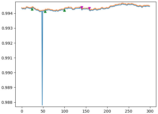
Figure 11.6 – Non-market price
To filter out at least bad ticks of this sort, let’s add a simple check: if the spread is greater than 10 pips, then skip this tick:
        if 'instrument_id' in tick.keys():
            bid = float(tick['bids'][0]['price'])
            ask = float(tick['asks'][0]['price'])
            if ask - bid < 0.001:
        tick_feed_0.put(tick)
Next, we need to implement the ticks aggregator. In our example, let’s form 10-second bars so that we can test our app and check if everything works correctly faster (without waiting for 1 minute or 1-hour bars to complete).
We will use only bid data to form bars for simplicity. Why is this possible? Because most of the time (except for the time around important news releases, bank settlement time, and the end/beginning of the week), the spread (the difference between the bid and ask) is more or less constant. So, if we want to emulate the real execution of orders, then we can use real bid and ask in the tick data stream, but for the trade logic, we can use bars built with only one price. Of course, for strategies of a certain kind, such as arbitrage, both bid and ask data are essential (and sometimes last trade along with the two), but now, we’re building a prototype that you will be able to customize the way you want when you are familiar with the approach in general.
For aggregating ticks into bars, we used almost the same code from Lesson 8, Data Visualization in FX Trading with Python, in the Plotting live tick data section, so not much commenting is required here:
data_resolution = 10
def getBarRealtime(resolution):
    last_sample_ts = datetime.now()
    bar = {'Open': 0, 'High': 0, 'Low': 0, 'Close': 0}
    while True:
        tick = tick_feed_0.get(block=True)
        if 'instrument_id' in tick.keys():
            ts = datetime.strptime(tick['timestamp'], "%Y-%m-%dT%H:%M:%S.%fZ")
            bid = float(tick['bids'][0]['price'])
            delta = ts - last_sample_ts
            bar['High'] = max([bar['High'], bid])
            bar['Low'] = min([bar['Low'], bid])
            bar['Close'] = bid
We created a bar, received a tick, and updated the bar’s high, low, and close values. Now, as soon as the time since the bar’s open is greater than or equal to 10 seconds, we start a new bar:
        if delta.seconds >= resolution - 1:
            if bar['Open'] != 0:
                bar_feed.put(bar)
                last_sample_ts = ts
                bar = {'Open': bid, 'High': bid, 'Low': bid, 'Close': bid}
        tick_feed_1.put(tick)
Note the last line of this function. It puts the same tick that’s received into tick_feed_1. This is done to trigger the next component, the trading logic:
def tradeLogic():
    while True:
        tick = tick_feed_1.get()
        try:
            bar = bar_feed.get(block=False)
            print('Got bar: ', bar)
Now, it’s time to add some trading logic.
Note
For testing purposes, we don’t care whether our test strategy is profitable or not – we only want to generate as many orders as possible to watch the emulated execution.
So, let’s implement the following simple logic:
- If the bar closes up (close > open), then sell
- If the bar closes down (close < open), then buy
With this “strategy”, we may expect many orders to be generated quickly, so we will be able to test our app without waiting for too long:
            ####################################
            #      trade logic starts here      #
            ####################################
            open = bar['Open']
            close = bar['Close']
            if close > open and System.market_position >= 0:
Here, we are checking that the bar’s closing price is greater than Open and also that the current consolidated market position is positive. We’re doing this because we don’t want to open multiple positions in the same direction. In other words, if we are already long in the market, we only wait for a short position to open, and vice versa:
                order = {}
                order['Type'] = 'Market'
                order['Price'] = close
                order['Side'] = 'Sell'
The following if…else statement checks whether we are opening the position for the first time. If we are, then we don’t have any current market position at the time of order generation, so in our example, the trading size is 10,000. But if there is already an open position and we want to open a new position in the opposite direction, then we should first close the existing position and then open the new one, which effectively requires twice the trading size. We have to use 10000 to close and 10000 to open a new position, which means a trading size of 2 * 10,000 = 20,000:
                if System.market_position == 0:
                    order['Size'] = 10000
                else:
                    order['Size'] = 20000
Finally, we must put the order into the order queue:
                orders_stream.put(order)
                print(order) # added for testing
Now, we must do exactly the opposite for the buy order:
            if close < open and System.market_position <= 0:
                order = {}
                order['Type'] = 'Market'
                order['Price'] = close
                order['Side'] = 'Buy'
                if System.market_position == 0:
                    order['Size'] = 10000
                else:
                    order['Size'] = 20000
                orders_stream.put(order)
                print(order)
            ####################################
            #      trade logic ends here      #
            ####################################
        except:
            pass
        tick_feed_2.put(tick)
Why do we use 10,000 base currency as the trading size?
If we trade EURUSD, a currency pair quoted with 4 or 5 digits, then buying or selling 10,000 euro (see Lesson 3, FX Market Overview from a Developer’s Standpoint, the Naming conventions section) would mean that 1 pip costs $1. Therefore, we can interpret the results of our tests both as in money and in pips. Since the FX market is highly leveraged (see the same in the Trade mechanics – again some terminology section in Lesson 3, FX Market Overview from a Developer’s Standpoint), it’s more convenient to calculate all PnL in pips and then scale it using leverage.
Note that this function uses a try…except statement. The reason is that we use two queues: tick_feed_1 to receive ticks and bar_feed to receive actual bars. However, ticks are only used in this function to trigger its execution (see the detailed explanation at the very beginning of this section), while bars are used to make actual trading decisions. The problem is that bars normally arrive far less frequently than ticks, so we can’t wait until there’s a bar in the bar_feed queue; otherwise, the normal execution of our app would be interrupted. That’s why we use the block = False attribute when reading from the bar_feed queue. However, if there’s a new tick in tick_feed_1, but there’s no bar in bar_feed, then the attempt to read from there would raise an exception. Therefore, we catch this exception and – in our current implementation – just do nothing, waiting for a new bar to arrive in the queue.
The final component of our trading app is order execution. We invoke this function by a tick received in tick_feed_2, where it’s put by tradeLogic():
def processOrders():
    while True:
        tick = tick_feed_2.get(block = True)
        current_price = float(tick['bids'][0]['price'])
With every received tick, we update the equity value of the trading system. Remember that equity in traders’ slang means the sum of all PnL values calculated on each tick or bar. If we have a long position and the current price is greater than the previous price, then the equity value increases on this tick/bar. The opposite is also true: if we have a short position and the current price is less than the previous price, then the equity value also increases on this tick/bar.
I believe you’ve got it: if we’re long and the price decreases or if we’re short and the price increases, then the equity decreases on this tick or bar. To calculate the actual equity value on the current tick, we multiply the difference in price between the current and the previous ticks by the market position value:
        System.equity += (current_price - System.last_price) * System.market_position
        System.equity_timeseries.append(System.equity)
        System.last_price = current_price
        print(tick['timestamp'], current_price, System.equity) # for testing purposes
Now, we start scanning the order queue and executing orders as they appear there. Note that we again use the block = False attribute, so we never wait for an order in the order queue: if there’s no order by the time a new tick is received, we just go ahead and proceed with the main loop:
        while True:
            try:
                order = orders_stream.get(block = False)
After we’ve received an order, we should do the risk management check: whether we have sufficient funds to execute this order. To calculate the available funds, we should add the current equity (positive or negative) to the initial capital and subtract the margin required for the currently open market position, which is the value of this market position divided by the leverage:
available_funds = (System.initial_capital + System.equity) * System.leverage - System.market_position / System.leverageHow to calculate available funds
The calculation of available funds that we are using in our code is not 100% correct. The problem is that it is possible to have a huge position in the market with some positive running PnL. In this case, our formula would say we have sufficient funds, but in reality, until this huge position is closed, we may not have enough money in the trading account. So, to be perfectly precise with this calculation, we should have introduced yet another variable to the system metadata that would account only for realized PnL (calculated by closed positions). However, we are not going to do this now, again for simplicity and transparency’s sake.
Now, if the order size is less than the available funds in the trading account, we can execute the order. A bit later, we will write a separate function that emulates the order execution. In production, this function can be replaced by an actual call to the broker’s API:
                if order['Size'] < available_funds:
                    emulateBrokerExecution(tick, order)
After attempting to execute the order, its status is changed either to ‘Executed’ or ‘Rejected’ (or any other status returned by your broker), so let’s decide what to do with it. Of course, if the order was successfully executed, we only update the strategy metadata (and print the result for testing purposes):
                if order['Status'] == 'Executed':
                    System.last_price = order['Executed Price']
                    print('Executed at ', str(System.last_price), 'current price = ', str(current_price), 'order price = ', str(order['Executed Price']))
                    if order['Side'] == 'Buy':
                        System.market_position = System.market_position + order['Size']
                    if order['Side'] == 'Sell':
                        System.market_position = System.market_position – order['Size']
If the order was rejected, we return it to the same order queue:
                elif order['Status'] == 'Rejected':
                    orders_stream.put(order)
Again, let me reiterate that, in reality, you may need more complex order handling, but it will depend on both the type of strategy you’re going to run and the types of order statuses provided by your broker.
Finally, we will just add the except clause so that nothing happens if there’s no order in the order queue:
            except:
                order = 'No order'
                break
We’re almost there! All we need to add now is the function that emulates the order execution at the broker. For the first version of our emulator, we will implement only the execution of market orders:
def emulateBrokerExecution(tick, order):
    if order['Type'] == 'Market':
        if order['Side'] == 'Buy':
It’s time for the final preflight check: making sure the market has sufficient liquidity before sending the order!
current_liquidity = float(tick['asks'][0]['quantity'])Don’t confuse bids and asks! If we buy, we check the liquidity at the offer (ask) and execute at the ask price, while if we sell, we use bids:
            price = float(tick['asks'][0]['price'])
            if order['Size'] <= current_liquidity:
                order['Executed Price'] = price
                order['Status'] = 'Executed'
            else:
                order['Status'] = 'Rejected'
        if order['Side'] == 'Sell':
            current_liquidity = float(tick['bids'][0]['quantity'])
            if order['Size'] <= current_liquidity:
                order['Executed Price'] = price
                order['Status'] = 'Executed'
            else:
                order['Status'] = 'Rejected'
Now, let’s review the components of the trading application we have added so far:
- Strategy metadata object (class tradingSystemMetadata)
- Queues for price data and orders (tick_feed_0, tick_feed_1, tick_feed_2, bar_feed, and orders_stream)
- A function that connects to the data source (LMAX_connect(url, subscription_msg))
- A function that forms bars from ticks (getBarRealtime())
- A function that makes trading decisions (tradeLogic())
- A function that processes orders (processOrders())
- A function that emulates order execution at the broker (emulateBrokerExecution(tick, order))
All we have to add to the very end of our code is a block that initializes and starts all four threads:
data_receiver_thread = threading.Thread(target = LMAX_connect, args = (url, subscription_msg))
incoming_price_thread = threading.Thread(target = getBarRealtime, args = (data_resolution,))
trading_thread = threading.Thread(target = tradeLogic)
ordering_thread = threading.Thread(target = processOrders)
data_receiver_thread.start()
incoming_price_thread.start()
trading_thread.start()
We have just developed our first trading app! It’s time to run it and check if it’s doing what we expect. I will run it and wait until the second order is executed (because I want to make sure that I submit correct orders both in case the strategy has an open position in the market and in case there’s no open position). If you repeated all these steps correctly, you should see an output like the following:
2022-12-12T12:03:20.000Z 1.05658 0.0
... (7 ticks omitted from output to save space)
2022-12-12T12:03:28.000Z 1.05664 0.0
We started at 12:03:20, so we received nine ticks (remember, LMAX doesn’t send actual ticks, but 1-second snapshots of market data). At the 10th second, we form a bar:
Got bar: {'Open': 1.05658, 'High': 1.05668, 'Low': 1.05658, 'Close': 1.05666}The bar’s close is greater than the bar’s open, so according to our test strategy logic, it is a signal to sell – and indeed, there’s an order that immediately follows the bar:
{'Type': 'Market', 'Price': 1.05666, 'Side': 'Sell', 'Size': 10000}Note that the order size is 10000 because we opened the position for the very first time and we don’t have open positions in the market yet. We check the 10th tick to make sure that its price equals the closing price of the bar and the order price:
2022-12-12T12:03:29.000Z 1.05666 0.0Now, we can see the execution report:
Executed at 1.05666 current price = 1.05666 order price = 1.05666So far, so good. Let’s wait for the next bar to form:
2022-12-12T12:03:30.000Z 1.05663 0.2999999999997449
... (7 ticks omitted from output to save space)
Got bar:  {'Open': 1.05666, 'High': 1.05666, 'Low': 1.05663, 'Close': 1.05665}
We’re lucky: the very next bar closed in the opposite direction (close is less than open), so it’s time to generate a buy order:
{'Type': 'Market', 'Price': 1.05665, 'Side': 'Buy', 'Size': 20000}Note that the order size this time is 20000: we need to close the currently open position of 10000 and then open a new one with the remaining 10000. Let’s check the tick price to make sure that the bar’s closing price and the order price are correct:
2022-12-12T12:03:38.000Z 1.05665 0.09999999999843467Great, everything looks good. Now, let’s proceed to order execution…
Executed at 1.05672 current price = 1.05665 order price = 1.05672Stop. What’s that? The last tick’s price was 1.05665, but the order is executed at 1.05672! Why?
This happens because we form bars using only bid prices and execute orders at actual market prices – bid for sell orders and ask for buy orders. The first order was a sell, so we used the bid price and all prices (bar, tick, order, and execution) coincided. But the second order was a buy, but we still used only the bid price to form a bar – that’s why we had the execution price greater than the bar’s closing price.
The importance of market spread
This issue perfectly illustrates the importance of taking spread (the difference between the bid and ask prices) into consideration when running tests. So many developers forget about it and run their testing using only bid prices – for simplicity, you know. These tests are not adequate for the real market, and quite frequently generate trade logic that is profitable only when you can buy and sell at the same price, effectively assuming the spread to be zero at all times. Now, you know how to avoid this trap and make sure your tests are always realistic.
Before we move on, let’s quickly review our code and see whether it meets the requirements outlined in Lesson 1, Developing Trading Strategies – Why They Are Different:
- It filters the incoming tick data feed and excludes non-market prices
- It is event-driven – it generates and executes orders as soon as the trade logic confirms a trade
- It does some basic risk management checks – position size, leverage, and available funds
- It is capable of emulating bad order execution and handling these situations
- And probably the main benefit: this code will never – never! – peek ahead, neither in testing nor in production (see Lesson 4, Trading Application – What’s Inside?, the Trading logic – this is where a small mistake may cost a fortune section)
So, we have developed a robust application suitable for serious production! Of course, it can be improved further, but its core will remain almost unchanged. However, we don’t have a tested strategy to run. How can we develop such a strategy?
This is when we can use the concept of backtesting, which we mentioned earlier, almost at the beginning of this app.
Leave a Reply